When it comes to finance, every investor wants to make sure they are putting their money in the right places. The last thing they need is having one of their debtors or investments go bankrupt! However, in the financial market, bankruptcy prediction or prediction of financial distress in companies has always been a challenging task. Fitzpatrick, in the 1930s compared 13 ratios that differentiated between failed and successful firms. Ever since then, a lot of research has been going on concerning this topic. Later on, in 1968 Altman went on to use Linear Discriminant Analysis (LDA) to develop a five-factor model to predict bankruptcy in manufacturing companies. Till date, this is a leading model in practical finance applications.
Let’s take a look at what this Linear Discriminant Analysis (LDA) is and why we use it.
What is Linear Discriminant Analysis?
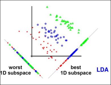
As the name suggests, Linear Discriminant Analysis tries to discriminate or differentiate between different classes. The primary aim of LDA is to find a vector in the system space that provides the best separation between elements of different classes when the elements are projected onto the vector.

Confused? Let me explain. As we discussed before, classifying an organization as potentially in distress or not depends upon a number of factors. Let us assume there are 13 factors, that govern whether an organization will go bankrupt or not. Processing all 13 factors can be computationally quite intensive; so it would be best if the 13 factors were reduced to say, just 5, such that these factors also provide a better distinction between the two classes (in distress or not in distress).
LDA does exactly that. It serves as a dimensionality reduction technique. Dimensionality reduction simply means plotting multi-dimensional data in just 2 or 3 dimensions. In other words, LDA reduces high dimensional data onto a lower-dimensional space.
As such, it is often used as a pre-processing step in machine learning and pattern classification tasks. As explained before, LDA also serves in finding vectors in the system that provide the best separation between the elements of different classes.
This greatly reduces calculations and allows us to get a better visual representation (If a 4-dimensional system can be reduced to just two dimensions, it will obviously help us visualize the system better).
How does LDA work and find the best vectors?
LDA’s main aim is to find the vectors that ensure a higher distance between the different classes, while simultaneously ensuring a lower variance (or spread) within each class. To do this, LDA uses Fisher’s ratio.
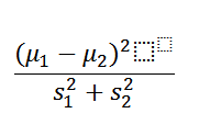
To find Fisher’s ratio, we need the means and the covariance matrices for each class. Our optimal vectors will be the ones that have the highest Fisher ratio. The idea is mainly to find the best trade-off between a higher distance between means and a more condensed in-class pattern, in order to get the best separation. The Fisher’s ratio takes both into account as follows (For a two-vector problem):

Ideally, the numerator (the difference between means of the classes) should be very large and the denominator (sum of squares of in-class variances) should be very small. That means our optimal vector will have the highest Fisher ratio.

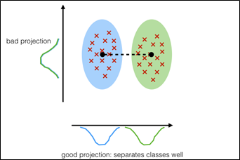
Why are both distance and scatter important?
If we only maximize the distance between the means, we get a lot of overlap between the two classes. But if we simultaneously optimize both criteria at the same time, we will get better separation.
So we now know how LDA works, but how does it apply to our bankruptcy problem?

The Z-score formula
Edward Altman proposed the Z-formula for predicting bankruptcy when dealing with multiple variables relating to companies. He used this formula to predict the probability of a company going into bankruptcy within two years. The Z-score uses a number of income and balance sheet values to measure the financial health of a firm. It is a linear combination of five business ratios, weighted by a set of 5 coefficients. The formula for the Z-score bankruptcy model is as follows:
Z = 0.012X1 + 0.014X2 + 0.033X3 + 0.006X4 + 0.999X5
Here, X1, X2, X3, X4 are in percentage points.
X1 = working capital / total assets
X2 = retained earnings / total assets
X3 = earnings before interest and taxes / total assets
X4 = market value of equity / total liabilities
X5 = sales / total assets
Altman found significant differences for each of these fundamental variables between the group of bankrupt borrowers and the group of non-bankrupt borrowers.
The above Z-score gives a credit rating that can be interpreted as follows:
Z > 2.99 – “Safe” Zone
1.81 < Z < 2.99 – “Grey” Zone
Z < 1.81 – “Distress” Zone
Conclusion
Linear Discriminant Analysis plays a huge role in predicting bankruptcy. Owing to its simplicity and benefits in reducing computational costs, it provides a great way for investors to look before they leap. As such, it is very important for data scientists and machine learning experts to have a thorough knowledge of this technique.

