Previously we spoke about decision trees and how they could be used in classification problems. Now we shift our focus onto regression trees. Regression trees are different in that they aim to predict an outcome that can be considered a real number (e.g. the price of a house, or the height of an individual). The term “regression” may sound familiar to you, and it should be. We see the term present itself in a very popular statistical technique called linear regression. Although linear regression and regression are not alike, the basic idea behind the “regression” part remains the same. Regression attempts to determine the relationship between one dependent variable and a series of independent variables.

In this article we hope to illustrate the difference between linear regression and regression trees in their usefulness, build our own regression tree and instantiate a regression tree in Python.

The Problem

Suppose we are scientists and have developed a brand new drug to treat the common flu.

However, we don’t know the optimal dosage for our patients. To investigate this problem we run a clinical trial with different dosages and measure how effective each dosage is. In the end we would like to accurately predict the efficiency of the drug at a certain dosage level.

Linear Regression

If we plot the results of the clinical trial in some hypothetical scenario, the data points may look similar to the graph below.

The data points in the plot above (Plot A) indicates that there is some positive correlation between drug dosage and drug efficiency. Meaning that in general, the higher the dose, the higher the efficiency. We could easily fit a straight line to this data with linear regression and use the line of best fit to draw predictions. For instance, a drug dosage of 23 mg has a predicted value of 63% efficiency. Unfortunately, data doesn’t always seem to present itself so well. More realistically, we might end up with data points being much noisier. This is seen in the plot below.

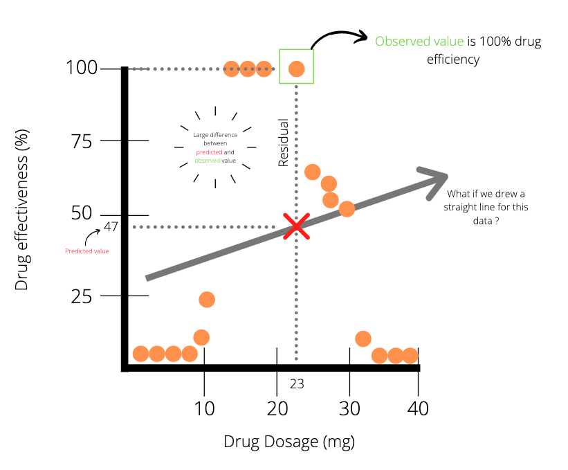
Applying linear regression to the data points (Plot B) above, we notice that there is a large difference between the predicted value and the actual value for a drug dosage of 23 mg. It seems evident that linear regression might not be the best method to model the data. Well, what other method could we use? Yep, you guessed it, it’s in the title: regression trees.

Regression Trees

Regression trees are similar to decision trees but have leaf nodes which represent real values. To illustrate regression trees we will start with a simple example. Don’t worry, we’ll get into the details shortly. For the root node of our tree we ask: “is dosage less than 14 mg?”. Then using the data points seen in Plot B, we should get a tree that looks similar to the one below.

If the answer to the question in the root node is “True”, then we are directed to the left node, otherwise we are directed to the right node, which carries on further.

For the time being let’s focus on the first leaf node on the left hand side: how did we get that value of 4.5%? Since we have a threshold of 14 in the root node, we look at observations which are less than 14 and calculate their average. In our case, the average of the first 6 observations is 4.5% (efficiency).

Once this first leaf node is complete we can apply the same process to the nodes on the right hand side. Each red block in the picture below represents a leaf node.

Let’s have a look at how we got the last leaf node on the right hand side (the leaf node with 100% efficiency)

We get the last leaf node on the right hand side by following the conditions set out by the nodes until the very end. If the dosage is more than 14 but less than 29 and 24, we are left with an interval which is highlighted in the picture below. The average drug effectiveness for the 4 observations in the red box is 100%.

So the tree uses the average value (100%) as the prediction value for dosages between 14.5 and 23.5.

Building our own Regression Tree

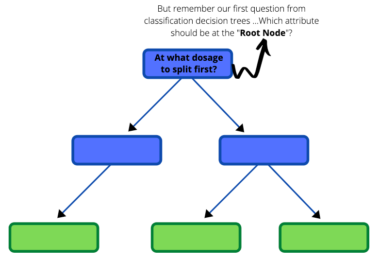
Now that we have gone through an example of what a regression tree looks like, let us develop one ourselves from the very beginning using the same unstructured data in Plot B. The first part of building a regression tree is deciding which threshold to have in the root node. Do you recall a similar question in the blog about decision trees?

To help us decide, we will first focus on the observations with the two smallest dosages. The average dosage between those two patients is 3 mg. We draw a vertical line at the point 3 to indicate a split in our data.

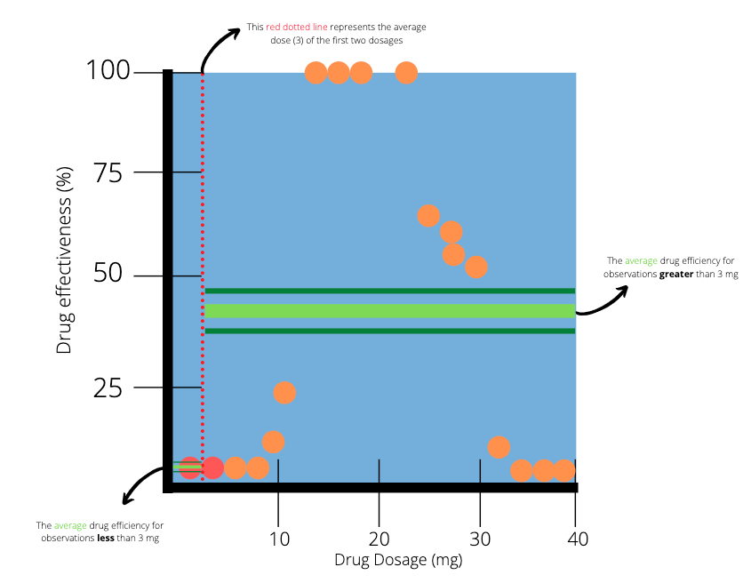
The two dots which are highlighted red represent the two smallest dosages. The red dotted line splits the data into two parts. The next step is to calculate the average efficiency of the observations on the left and right hand side of the red dotted line. On the left hand side (less than 3 mg), there is only one observation, which results in an average of 0%. On the right hand side (greater than 3mg), there are many observations with an average of 38.8.

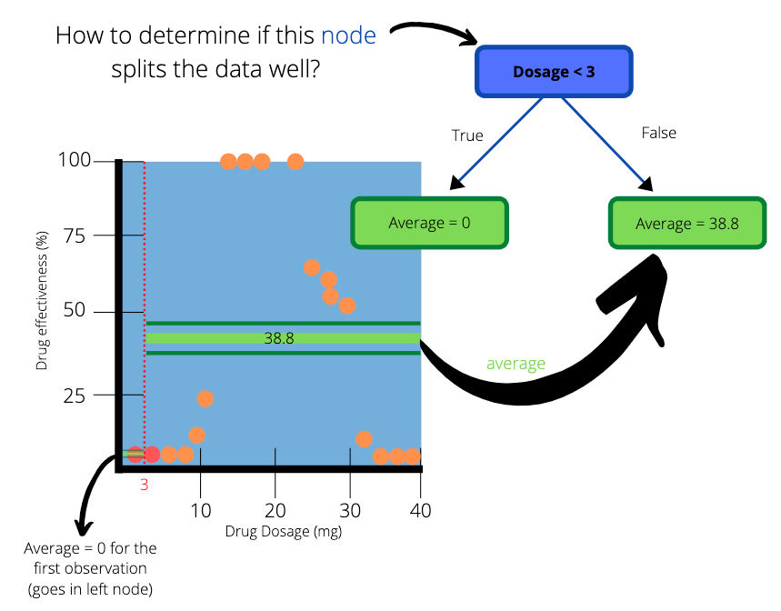
We create a simple tree with “Dosage < 3” as the root node and two subsequent leaf nodes. The average on the left hand side of the dotted line goes into the left leaf node and the average on the right hand side goes to the right leaf node. The values in the leaf nodes are the predictions that this simple tree will make for drug effectiveness.

How to determine how well our simple tree splits the data ?

The left leaf node has predicted the outcome perfectly. The actual efficiency for dosages less than 3mg is 0% and our tree predicted it as such. But how do we check the accuracy of the right hand side when there are so many observations to consider?

We can use a method that is common in linear regression:

Sum of Squared Residuals (SSR)

A residual is a measure of the distance from a data point to a regression line. SSR measures the overall difference between our data and the values predicted by our regression tree. Generally, a lower SSR indicates that the regression model can better explain the data while a higher SSR indicates that the model poorly explains the data. The formula of SSR:

We can visualise the residuals of our simple tree by constructing lines from the observed to the predicted value. Notice again that on the left hand side the predicted value is equal to the observed value.

We can use the residuals to quantify the quality of the predictions made by our simple tree. Next we calculate the SSR for the tree by adding the SSR of the left and right leaf nodes.

We get a total SSR value of 27.5 for the tree. The entire process is then applied to the second and third lowest observations, the third and fourth lowest observations and so on..

Once we have calculated all the SSR values for the trees made by the pairs of observations, we can plot the SSR values as a function of dosage threshold.

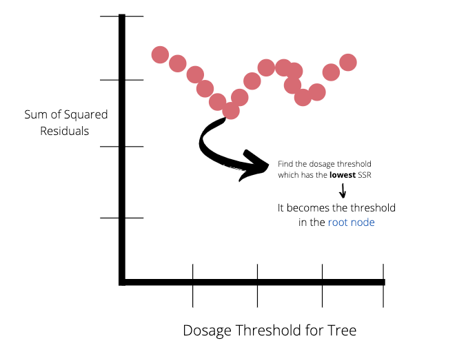
The lowest SSR value represents the dosage threshold which will be at the root node of the tree. In this case the lowest SSR value is 14.

Once the root node has been decide, the data will be split up into a left and right node. These nodes also require an optimal threshold to split the data further. How do we go about choosing these thresholds? The same process which was applied to obtain the root node is now applied to the remaining nodes of the tree. Each node should have a threshold which represents the lowest SSR value available. Once the data cannot be split further (only one observation in the train data) or there it is redundant to split (if all observations have the same value), the node itself becomes the leaf node.

Building Regression Trees in Python

Here we will have a quick look at building a regression tree in Python with the Sklearn package

About the Dataset

We will be generating a random data set to represent the clinical trail example that was discussed earlier.

Note: In the notebook we do not clean the data. The reason for this is that the purpose of the blog is to illustrate how to run a regression tree classifier and not show data cleaning techniques. The onus is on the reader to properly clean the data. Data cleaning and preparation is an extremely important phase within the data science world and should not be overlooked.

Import the necessary libraries

import pandas as pd
import numpy as np
from sklearn.tree import DecisionTreeRegressor
from sklearn.model_selection import train_test_split
import matplotlib.pyplot as plt

Create a Random Data Set

rng = np.random.RandomState(1)
X = np.sort(5 * rng.rand(80, 1), axis=0)
y = np.sin(X).ravel()
y[::5] += 3 * (0.5 - rng.rand(16))

X and Y arrays are generated using the code above. The user can select their own parameters for reproducibility purposes.

View the data set

plt.figure()
plt.xlabel("Dosage (mg)")
plt.ylabel("Efficiency")
plt.scatter(X, y)
plt.show()

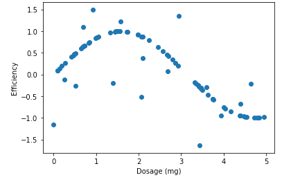
Unlike the dependent variable in the example, we will consider some arbitrary measure for the efficiency of the drug dosages. Notice the trend in the plot. The optimal dosage seems to be around 1.8mg. Our goal is to predict the efficiency of a drug given the dosage, all with the help of regression trees.

Create Training and Testing Data Sets

Next step is to split our data into training and testing data sets. The training data set is used to train/create our regression tree. Then the regression tree is tested on our testing data set to see how well it performs on unseen data. We use the train_test_split function from Sklearn.model_selection to achieve this.

# Create the training and test sets
X_train, X_test, y_train, y_test = train_test_split(X, y, test_size=0.2, random_state=123)

Instantiate the Regression Tree Classifier

Here we instantiate the regression tree classifier and set the parameters. All the parameters are detailed here. We will only go through a few of them:

1) Criterion{“mse”, “friedman_mse”, “mae”}, default=”mse”: The function to measure the quality of a split. Supported criteria are “mse” for the mean squared error, which is equal to variance reduction as feature selection criterion and minimizes the L2 loss using the mean of each terminal node, “friedman_mse”, which uses mean squared error with Friedman’s improvement score for potential splits, and “mae” for the mean absolute error, which minimizes the L1 loss using the median of each terminal node.

2) max_depth: int, default=None: The maximum depth of the tree. If None, then nodes are expanded until all leaves are pure or until all leaves contain less than min_samples_split samples.

3) min_samples_split: int or float, default=2: The minimum number of samples required to split an internal node

The parameters may be tuned in order to find the best regression tree in terms of some chosen criterion. A grid search is a popular method used to return the optimal parameters.

clf = DecisionTreeRegressor(max_depth=2)

Fit the Classifier to the Training Set

clf.fit(X_train, y_train)

Predict the Target Variable of the Test Set: y_pred

In our case it’s drug efficiency.

y_pred = clf.predict(X_test)

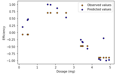
View the predicted values versus the observed values in the test data set.

plt.figure()
plt.scatter(X_test, y_pred, s=20, edgecolor="black",
            c="darkorange", label="Observed values")
plt.scatter(X_test, y_test, s=20, edgecolor="black",
            c="blue", label="Predicted values")plt.xlabel("Dosage (mg)")
plt.ylabel("Efficiency")
plt.title("Decision Tree Regression")
plt.legend()
plt.show()

Caveat

Regression trees with a large depth value have a high probability of over-fitting the training data set. When this happens, the model is unlikely to perform well when exposed to new and unseen data. To overcome this obstacle one could decrease the maximum depth of the tree or increase the minimum number of samples required to split an internal node. Another popular technique is pruning the regression tree. Pruning is a technique that reduces the size of regression by removing sections of the tree that provide little power to classify instances.

https://corporatefinanceinstitute.com/resources/knowledge/other/sum-of-squares/

StatQuest with Josh Starmer

https://scikit-learn.org/stable/auto_examples/tree/plot_tree_regression.html