First of all it is really interesting to work with mathematical problems. Right? I know the answer can be yes and no. Still applying maths on real world problems for optimisations, modelling will be really good. I started to do this recently and see how things works for me. So this blog is a part of my learning and it is to understand how computational complexity for convolution can be reduced using Fourier Transform techniques. I will try to go in detail.

Let’s see what Wikipedia has to say about Fourier Transform.

Is it confusing? If yes lets see how it helps us.

The algorithm helps in such a way that it allows us to split the input signal that is spread in time (Like in the image above) into the number of frequencies of length, amplitude and phase so that all these frequencies together can reform the original signal.

So it actually converts the data information of time domain into domain of frequencies and also backwards.

Let’s work with an analogy. We usually make tea right. Ingredients of tea are milk, tea powder, sugar and water. Here fourier transform helps us to split out the ingredients to 4 different bottles with each in each one. This is what FT does — it splits the whole input into its ingredients.

let’s start working on it.

Our main aim is to use fourier transform to reduce the computational complexity for convolution. There are lots and lots of applications in computing, physics, sound mixing etc..

You know how convolution works, we take a filter(kernel) and we will be having an image so what happens is we hover the filter above the image pixels and multiply and sum them up. After that the filter move to the next set of pixels and multiply then sum.

Woah! There will be lots of multiplication and computational complexity.

How can we solve this using Fourier Transform?

There is a nice and awesome property of Fourier transform related to convolution. This mentions that convolution of two signals is equal to the multiplication of their Fourier transforms. Yeah! So instead of multiplying throughout the image with the kernel we could take the Fourier transform of it and just get a bit wise multiplication. This can even be applied in convolutional neural networks also. Before the convolutional layer transform the input and kernel to frequency domain then multiply then convert back. Even though it deals with transforming and reverse transforming still it is computationally less expensive.

Before moving onto the implementation and application let us first see and understand what is the difference of Fourier Transform and Fast Fourier Transform and also why we prefer to do Fast Fourier Transform?.

This is the equation of Fourier Transform.

In Fourier Transform we multiply each of the signal value [n] with e raised to some function of n. So here comes N (multiplications) x N (additions) thus the computational complexity in Big-O notation is O(N²)

Fast Fourier transform is a method to find Fourier transform in a way that minimise this complexity by a strategy called divide and conquer because of this the computation complexity will be reduced to O(NlogN). Check the below table how it helps us in finding fourier transform.

So let’s consider a case where it take 1 nano second for a operation. It would take Fast Fourier Transform to complete it in 30s. However regular algorithm will need more than 10¹⁸ => 31.2 years.

If you want to read more about the Fast Fourier Transform computation complexity and simple implementations, check out the below link.

Applying Fourier Transform in Image Processing.

We will be following these steps.
1) Fast Fourier Transform to transform image to frequency domain.
2) Moving the origin to centre for better visualisation and understanding.
3) Apply filters to filter out frequencies.
4) Reversing the operation did in step 2
5) Inverse transform using Inverse Fast Fourier Transformation to get image back from the frequency domain.

Some Analysis

• Digital images are not continuous so we use DFT instead of Fourier transform.

• Ordinary DFT is slow so we chose FFT. (reason mentioned above)

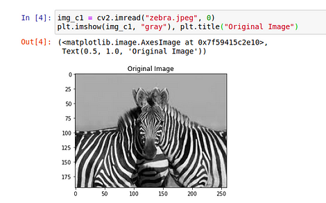
1. First we have to read the image. Here we are using CV package to read the image. Now the image is loaded in grey scale format.

2. Now we are going to apply FFT from numpy package. This means that we are taking the discrete image pixel values and are transforming it to a frequency domain and visualising it. The whole information is reserved but transformed to another domain.

Here you can see that there are white spots over corners which represents the low frequency components.

3. In this step we take the origin from corner to centre. This results in such a way that the centre part contains the low frequency components where as other contains high frequency.

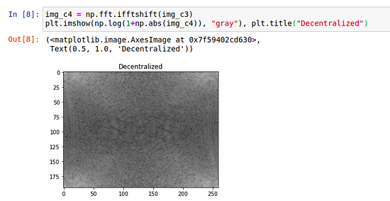
4. As the next step we are going to decentralise the origin back to where it belong to so that we can convert the image in frequency domain back to what we had.

5. Final step, here we reverse back the image from the frequency domain by using inverse fourier transformation.

Image Processing

Low frequencies in images are pixel values that are changing slowly that means the smooth areas with slightly color changing. Similarly high frequencies are pixels whose values are changing fast. This include edges with rapid changes in pixel values. So while we need to process the images in various methods we need to apply various filters mask etc in applications like edge detection, smoothing, removing noise etc.. Common filters that we use are High Pass filter, Low Pass filter, Ideal filter, Butterworth filter etc..

Let’s try some processing..

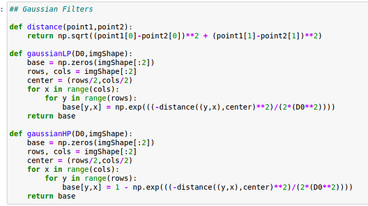
We are going to work on a Gaussian Filter now.

In this case formula for Gaussian low pass filter where D₀ is a positive constant and D(u, v) is the distance between a point (u, v) in the frequency domain and the center of the frequency rectangle. Formula for Gaussian high pass filter where D₀ is a positive constant and D(u, v) is the distance between a point (u, v) in the frequency domain and the center of the frequency rectangle. These equations are shown above.

How do these filters works?

So in low pass filter only the centre portion has high values which diminishes going beyond centre. As we have already seen the centre contains low frequency components. Thus it removes high frequency component when we multiply and keep low frequency. The opposite happens in the other case.

Using this filters now our process is to multiply these filters along with image instead of convolving the filter to the entire matrix. (This is how Fourier Transform helps us in computation)

Now lets do the process again.

1. Convert image to Discrete Fourier Transform here we use Fast Fourier Transform.
2. Shift the origin to centre.
3. Apply filter by multiplying filter with fourier representation of image.
4. Reverse the shift.
5. Inverse fourier transform for image.

In the above code snippet we do the steps above and we got the result as observed.

Checkout the Github repo below.