Here are 6 classification algorithms to predict mortality with Heart Failure; Random Forest, Logistic Regression, KNN, Decision Tree, SVM, and Naive Bayes to find the best Algorithm.

Introduction
In this blog post, I will use 6 different classification algorithms to predict mortality with heart failure.
To do so, we will use classification algorithms.
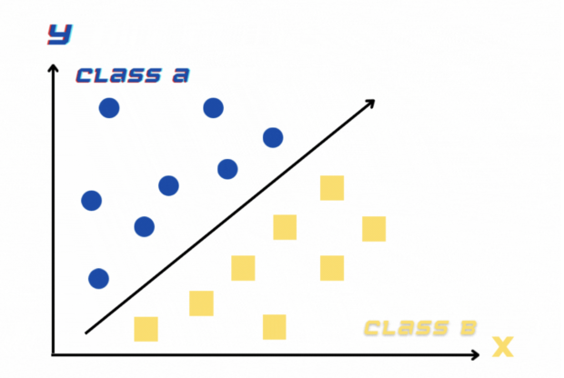
Here are the algorithms that I will use;
- Random Forest
- Logistic Regression
- KNN
- Decision Tree
- SVM
- Naive Bayes
And after that, I will compare the results according to the;
- Accuracy
- Precision
- Recall
- F1 score.
That will be longer than my other blog post, yet after reading this article, you will probably have a huge knowledge about Machine Learning Classification Algorithms and Evaluation metrics.
If you want to know more about Machine Learning terms, here is my blog post, Machine Learning A-Z Briefly Explained.
Now let’s start with the data.
Data Exploration
Here is the dataset from the UCI Machine Learning repository, which is an open-source website, you can reach many other datasets, which are specifically classified according to task( Regression, Classification), attribute types(categorical, numerical ), and more.
Or if you want to find out where to find free resources To download datasets.
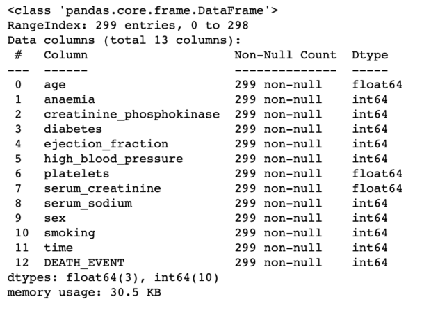
Now, this dataset, contains the medical records of 299 patients who had heart failure and there are 13 clinical features exist, which are;
Age(years)Anemia: Decrease of red blood cells or hemoglobin (boolean)High blood pressure: If the patient has hypertension (boolean)Creatinine phosphokinase (CPK): Level of the CPK enzyme in the blood (mcg/L)Diabetes: If the patient has diabetes (boolean)Ejection fraction: Percentage of blood leaving the heart at each contraction (percentage)Platelets: Platelets in the blood (kiloplatelets/mL)Sex: Woman or man (binary)Serum creatinine: Level of serum creatinine in the blood (mg/dL)Serum sodium: Level of serum sodium in the blood (mEq/L)Smoking: if the patient smokes or not (boolean)Time: follow-up period (days)[ target ] Death event: If the patient deceased during the follow-up period (boolean)
After loading the data, let’s have a first glance at the data.

To apply a machine learning algorithm, you have to be sure about data types, and check whether columns have non-null values or not.
Sometimes, our data set can be sorted along with one specific column. That’s why I will use the sample method to find out.
By the way, if you want to view the source code of this project, subscribe to me here and I will send the PDF contains codes with the description.
Now, let’s continue. Here are the 5 random sample rows from the dataset. Do not remember, if you run the code, the rows will be completely different because these functions return rows randomly.

Now let’s look at the value counts from high blood pressure. I know, how many options will exist for this column(2) yet checking makes me feel competent about the data.

Yes, it looks like, we have 105 patients who have high blood pressure and 194 patients who have not.
Let’s look at the smoking value counts.

I think it’s enough with data exploration.
Let’s make data visualization a little bit.
Of course, this part can be extended due to the needs of your project.
Here is the blog post, which contains examples of data analysis with python, especially using the pandas library.
Data Visualization
If you want to check out the distribution of the features, to eliminate them or do outlier detection.

Of course, this graph is just informative. If you want to look closer to detect outliers, you have to draw a graph each.

Now, let’s get into the feature selection part.
By the way, Matplotlib and seaborn are highly effective data visualization frameworks. If you want to know more about them, here is my article, about Data Visualization for Machine Learning with Python.
Feature Selection
PCA
Okey, not let’s select our features.
By doing PCA, actually we can find the n feature counts to explain the x percentage of the data frame.
Here, It looks like, about 8 features will be enough for us to explain %80 of the dataset.

Correlation Graph
Related features, will ruin the performance of our model so after doing PCA, let’s draw a correlation map to eliminate the correlated features.
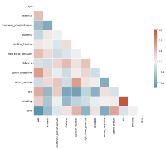
Here, you can see sex and smoking look highly correlated.
The main purpose of this article is to compare the results of the classification algorithms, that’s why I won’t eliminate both of them, but you can in your model.
Model Building
Now it is time to build your machine learning model. To do that, first, we have to split the data.
Train- Test Split
Evaluating your model’s performance on the data that the model does not know, is the crucial part of the machine learning model. To do that, generally, we split the data 80/20.
Yet another technique is used to evaluate the machine learning model, which is cross-validation. Cross-validation is used to select the best machine-learning model among your options. It is sometimes called a dev-set, for further information you can search Andrew NG’s videos, which are highly informative.
Now let’s get into the model evaluation metrics.
Model Evaluation Metrics
Now let’s find out the classification model evaluation metrics.
Precision
If you predict Positive, what is the percentage of making accurate choices?
Recall
True Positive Rate against all positive.
F1 Score
The harmonic mean of the recall and the precision
For more about classification, here is my post: Classification A-Z Briefly Explained.
Here are the formula of precision, recall, and f1 score.


Random Forest Classifier
Our first classification algorithm is random forest.
After applying this algorithm, here are the results.
If you want to view the source code, please subscribe to me here for FREE.
I will send you the PDF, which includes the code with an explanation.

Now, let’s continue.
Logistic Regression
Here is another example of classification.
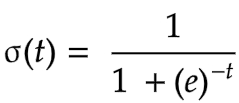
Logistic regression uses the sigmoid function to do binary classification.

This one’s accuracy and precision look higher.
Let’s continue searching for the best model.
KNN
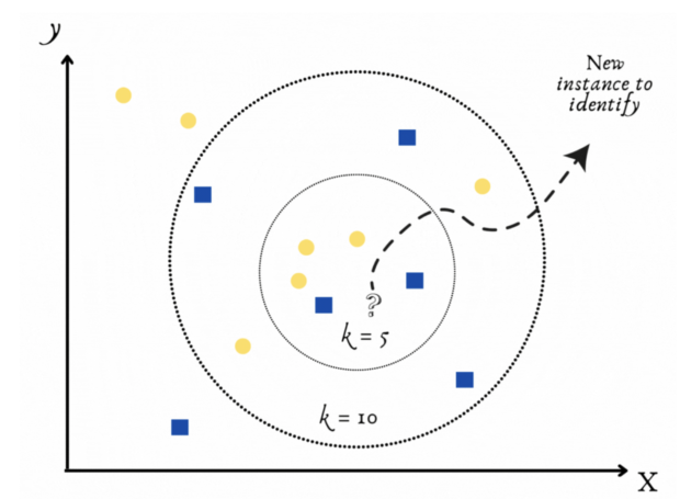
Okey, now let’s apply the K-nearest neighbor and see the results.
But when applying Knn, you have to select the “K”, which is the number of the neighbor you will choose.
To do that, using a loop looks like the best way.

Now, it looks like 2 has the best accuracy, yet eliminating human intervention, let’s find out the best model by using the code.

After choosing k=2, here is the accuracy. It looks like K-NN does not work well. But maybe we have to eliminate correlated features of normalization, of course, these operations can be varied.

Fantastic, let’s continue.
Decision Tree
Now it is time to apply the decision tree. Yet we have to find the best depth score to do that.
So when applying our model, it is important to test different depths.

And to find the best depth among the results, let’s keep continue automating.

Okay, now we find the best-performance depth. Let’s find out the accuracy.

Excellent, let’s continue.
Support Vector Machine
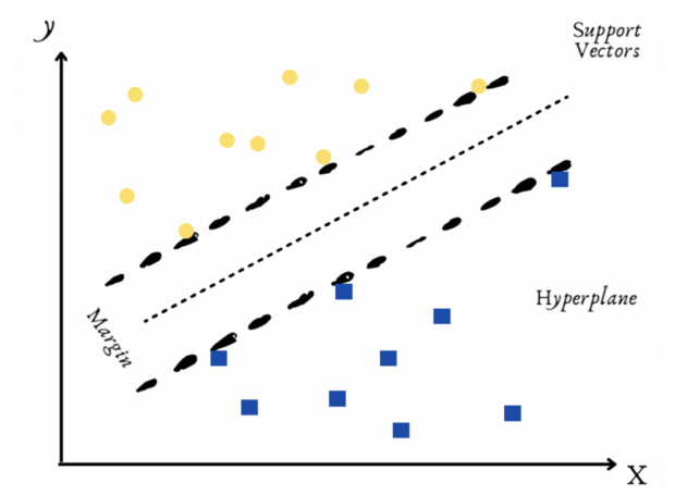
Now to apply the SVM algorithm, we have to select the kernel type. This kernel type will affect our result so we will iterate to find the kernel type, which returns the best f1 scored model.

Okey, we will use linear kernel.
Let’s find the accuracy, precision, recall, and f1_score with a linear kernel.

Naive Bayes
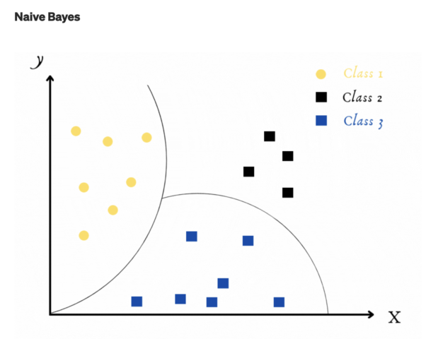
Now, Naive Bayes will be our final model.
Do you know why naive Bayes is called naive?
Because the algorithm assumes that each input variables are independent. Of course, this assumption is impossible when using real-life data. That makes our algorithm “naive.”
Okay, let’s continue.

Prediction Dictionary
Now after finishing the model search. Let’s save whole outputs into one data frame, which will give us a to chance of evaluation together.
After that now let’s find out the most accurate model.
Most Accurate Model

Model with Highest Precision

Model with Highest Recall

Model with Highest F1 Score

Conclusion
Now, the intended metric might differ according to your project needs. You might find out the most accurate model, or the model with the highest recall.
This is how, you can find out the best model, which will serve the needs of your project.
If you want me to send the source code PDF with an explanation for FREE, please subscribe to me here.
Thanks for reading my article!
I tend to send 1 or 2 E-Mails per week, if you also want a free Numpy CheetSheet, here is the link for you!
If you still are not a member of Medium and are eager to learn by reading, here is my referral link.
“Machine learning is the last invention that humanity will ever need to make.” Nick Bostrom

