How does a Machine Learn?

This article is for tech enthusiasts’ who are always inquisitive. I will give an introduction on Machine Learning, starting with a brief introduction about the concept of Machine Learning and then dive into how exactly machine ‘learns’ from the data given and produce the desired results. I have chosen Linear Regression model for demonstration purposes because a lot of people have used it in their day-to-day analysis. I will keep the mathematics as simple as possible so that it can be comprehended by a wider audience.

What is Machine Learning?

As the name suggests, Machine Learning is a concept where a machine (mostly a computer) learns from the data. It is basically an algorithm which is designed such that when it is fed with data, it can pick up patterns. The machine ‘learns’ some features about the data, some hidden patterns which might not be obvious to a human, some function or rules which can be used to make useful predictions.

Why is it necessary?

In today’s era, there’s a huge amount of data being generated through all sorts of activities every second. Your mobile usage creates data. Your daily commute to office creates data. In your office, employee records are data. Onboarding generates data. Your communications creat audio data. Your transactions create data. Your social media posts and visits create data. Surfing on YouTube creates data etc..etc. You can access this data, try to understand it and gather some useful insights. But! Imagine if you can somehow realise the usage patterns of a customer on YouTube. Can you recommend him some amazing videos based on his likings? Will this be helpful for him? Can it enhance his overall experience? E-commerce websites like Amazon, Flipkart and video streaming sites like Youtube, Netflix, use machine learning on a daily basis to improve customer experience. Imagine that you have all the tweets on a bank’s customer care page in Twitter. If you can somehow analyse these tweets and find out where are the customers facing an issue, and to what degree, will that be useful? Can banks leverage this insight to improve their services? Have you wondered how does Swiggy or Zomato tell you the time that your food will take to reach your doorsteps? How does an airline annoyingly increase the fares of the flight that you’ve been searching for some time? Well, the answer to ‘somehow’ is through Machine Learning. Considering the volume of data that is being generated, you simply exclude the possibility of a human trying to analyse these data. Lets now try to understand how does machine learning makes this possible. For this, I will take Linear Regression as my base, since everyone has used it occasionally to make predictions. Linear regression is a simple application of machine learning.

Problem Statement

Let’s say, there is a bank that gives discounts to its customers on a certain product based on how much money they have deposited in the bank. Given the historical customer data, we want to predict what discount should the bank give to a customer if he has deposited ‘x’ amount of money.

Solution

Our intuition tells us that the more the amount of money deposited, the more will be the discount percentage. We have a database of customers with their deposit amounts as well as the discounts given to them in the past. The deposit amount will be denoted as ‘X’ and is an independent variable. The discount percentage will be represented as ‘Y’ and is a dependent variable since it depends on the deposit amount. This is a snapshot of our data. 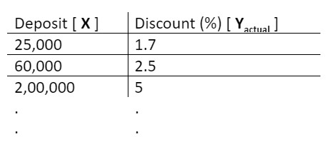Note: I will be denoting the discounts present in the data as Y_actual since these are the actual values observed in the data historically. So the machine has all the historical values of X and their corresponding Y Its goal is to figure out the hidden relationship between these two variables using the historical data, so that using this relationship, we can find out what discount should the bank give to a new customer based on his deposit. Therefore, to accomplish this task, the model will first assume a relation between Y and X as follows:

                    Y_model = m*X + c

                    Y_model = the discount that the model predicts

                    m = slope of the line

                    c = intercept of the line

                    X = deposit amount

This is an equation of a straight line with slope as m and intercept as c. This is what we want right? Some sort of equation where if we feed in a deposit amount (X), we can get the discount percentage (Y) based on historical trends. But how does a computer or machine know what values of m and c to use? The machine will need to ‘learn’ the values of m and c from the data. This is where the magic happens. Let's see how the machine uses the data to learn m and c. Initially, the model will assume some random values of m and c. It then calculates the error that is caused due to the assumptions by comparing the model output (Y_model) with the actual discount (Y_actual) from the data. Error: (Y_actual - Y_model)² Note: The error is squared so that negative and positive errors do not cancel out each other. Using the assumed m and c values, the machine calculates the discount percent(Y_model) for all the deposit amounts(X) in the historical data and then finds the error by comparing it with the actual discount(Y_actual) given to the customer. The overall error is the sum of all these individual errors. Now the machine’s goal is to basically find such m and c which will lead to a minimum overall error.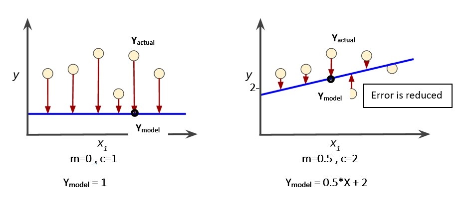   In the above figure, the blue straight lines are what the model has predicted based on the data points shown as round dots. The round dots are the actual data. The corresponding point on the blue line is what the model thinks it should be based on X. The difference between the actual data (round circles) and the corresponding point on the blue line is the error! So as you can see, the error is reduced in the second graph. The model will learn the values of m and c through a technique called Gradient Descent. The technique here is as follows:

• Look at this function: Overall Error = ∑ (Y_actual – Y_model)²
• Overall Error = ∑(Y_actual - (m*X + c) )² Note: we are replacing Y_modelwith m*X + c

• So our overall error depends only on m and c after you feed in all the values of X and Y_actual from the data.

Let's take some time and visualize this in a 3D graph. [caption id="attachment_15019" align="aligncenter" width="970"] Source: Stackoverflow[/caption] With the initial random guess, the model is somewhere on the surface. It ultimately needs to reach to the bottom where the overall error is minimum. The model needs to take guesses and take steps down the surface towards the bottom. But the guesses need to be intelligent! We know that at the bottom of the curve, the slope of the line will be zero! And the slope of the line keeps increasing as we go to the top of the blue surface. The model will first find the slope of the point where it initially is. Depending on the magnitude of the slope it will descend down the surface. If the slope is too large, it comes to know that it is way up on the surface and needs to take bigger steps to reach down. Whereas if the slope is near zero, the model comes to know that it is near the Minimum error point, and it should take small steps. Once it knows how big or small step to take, it guesses new values of m and c such that the values lead the model down the surface. Ultimately after a few guesses, the model reaches the bottom of the surface and the overall error is minimized! The values of m and c when the machine reaches the bottom, are finalized and the relationship m*X+c is defined using these values. That’s it! Now you have the required relation established between Y and X. So briefing everything up, first, the machine gets the historical data. It then formulates the overall error which it needs to minimize. Starting by assuming random values of m & c, it uses the technique of gradient descent to reach the bottom of the curve, and on its way keeps learning new and better values of m and c. Once the overall error is minimized, it uses the m and c values to define the final relation between Y and X. I hope you got some idea about how a machine learns from the data! Linear Regression was just the easiest implementation of the Machine Learning concept. As you come across different models, you would notice some more interesting ways to make the model learn from different types of data. Can you think how would a machine learn from images? .