Introduction to Time Series Forecasting of Stock Prices with Python

In this simple tutorial, we will have a look at applying a time series model to stock prices. More specifically, a non-seasonal ARIMA model. We implement a grid search to select the optimal parameters for the model and forecast the next 12 months. 

The ARIMA (p,d,q) model

The acronym ARIMA stands for Auto-Regressive Integrated Moving Average and is one of the most common tools for forecasting a time series. Before we can apply ARIMA to a time series, the time series needs to be stationary. Stationary implies that the statistical properties are all constant over time, i.e there is no trend in the time series. Stationarity of a time series is often obtained by differencing the time series, and a time series that needs to be differenced is said to be an “integrated” version of a stationary series, hence the “I” in ARIMA. Once stationarity has been reached by a certain number of differences, we are left to determine the number of autoregressive terms (parameter p) and the number of lagged forecast errors in the prediction equation (parameter q). The number of lagged forecast errors is also often referred to as the “moving average”.

Downloading the Data

I will be using Amazon’s historical monthly stock price, which can be downloaded as a CSV file at the link. Yahoo finance has various other stocks to choose from.

Import the necessary libraries

import numpy as np
import pandas as pd
import matplotlib.pyplot as plt
%matplotlib inline
from statsmodels.tools.eval_measures import rmse
import seaborn as sns
import statsmodels.api as sm
import itertools
from statsmodels.tsa.arima_model import ARIMA, ARMA
import warnings
warnings.filterwarnings("ignore")

Now it’s time to import the dataset and view it. We do so using the panda's library and its read_csv function.

data = pd.read_csv('filepath')
data.head()

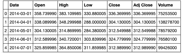We are only interested in the “Close” price. Also, we need to set the date as the index for the data frame.

df = data[['Date','Close']]
df.Date = pd.to_datetime(df.Date)
df = df.set_index("Date")

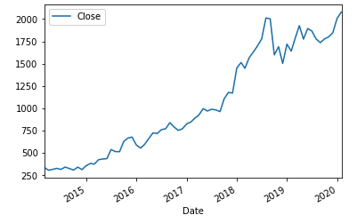
Now that we have preprocessed our data, we can view the data as a line plot. Visualising our data is an important part of exploratory data analysis.

df.plot(style="-")

When fitting an ARIMA model, we aim to find the values of our parameters p,d and q which optimise or minimise a certain metric of interest. There are many methods to achieve this goal and yet the correct parametrization of ARIMA models can be a tedious process that requires statistical expertise and time. In this tutorial, we hope to overcome this issue by writing a grid search algorithm in python to select the optimal parameter values for our ARIMA(p,d,q) time series model. The use of a “grid search” is to iteratively explore different combinations of parameters. For each combination of parameters, we fit an ARIMA model with the SARIMAX() function and assess its overall performance. Once we have explored the entire domain of parameters, our optimal set of parameters will be the one that yields the best performance for our criteria of interest. In this scenario, our criteria of interest is the Akaike information criterion (AIC). The AIC measures how well a model fits the data while taking into account the overall complexity of the model. We are therefore interested in finding a model that returns the lowest AIC value. In the code below we define the parameters and generate all possible combinations of the parameters.

# Define the p, d and q parameters to take any value between 0 and 3
p = d = q = range(0, 3)
# Generate all different combinations of p, q and q
pdq = list(itertools.product(p, d, q))

In the next few lines of code, the SARIMAX() function is applied to all combinations of parameters and the model with the lowest AIC is printed.

warnings.filterwarnings("ignore")
aic= []
parameters = []
for param in pdq:
  #for param in pdq:
      try:
          mod = sm.tsa.statespace.SARIMAX(df, order=param,       
enforce_stationarity=True, enforce_invertibility=True)
         
          results = mod.fit()
          # save results in lists
          aic.append(results.aic)
          parameters.append(param)
          #seasonal_param.append(param_seasonal)
print('ARIMA{} - AIC:{}'.format(param, results.aic))
      except:
          continue
# find lowest aic          
index_min = min(range(len(aic)), key=aic.__getitem__)           

print('The optimal model is: ARIMA{} -AIC{}'.format(parameters[index_min], aic[index_min]))

The output is: The optimal model is: ARIMA(0, 2, 1) — AIC:853.8946396688659 The next step is to fit the ARIMA(0,2,1) model to our time series.

model = ARIMA(df, order=parameters[index_min])
model_fit = model.fit(disp=0) print(model_fit.summary())

Finally, we can forecast the next 12 months and visualise the data points thereafter.

model_fit.plot_predict(start=2, end=len(df)+12)
plt.show()

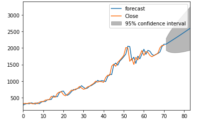There we have it! Your first stock prediction algorithm. However, please note that it is extremely difficult to “time” the market and accurately forecast stock prices. This tutorial should not be seen as trading advice and the purchasing/selling of stocks is done at your own risk.