Why My Self-Corrective RAG Kept Wasting Compute Until I Fixed One Number

Some developer mistakes are easy to make and hard to see. I made this one while working on a personal experiment.

 It’s not a bug. My code runs perfectly. My system was doing exactly what I designed it to do. But the problem was that my design was incorrect.

So I made that mistake while I was working with a self-corrective RAG system that was inspired by CRAG (Corrective Retrieval-Augmented Generation). 

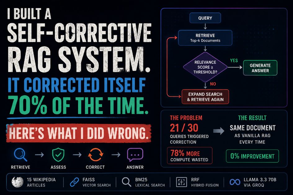
In this, the system had a relevance gate, which means after we retrieve the documents, it will score each one, and if the confidence is too low, it will expand the search and try again.

This is what happened with me: My design triggered corrections on 21 out of 30 queries. That means, it spent 78% more compute on those corrections. Well, that’s a lot of extra work I'm putting into it, but the surprising thing is that, still, it returned the same document as vanilla RAG every single time.

After digging inside my code base, I realize there's nothing wrong with my system — Threshold is the real culprit.

This is the story of that experiment — what I built, what went wrong, and what happened when I fixed it.

The Setup

Before anything else, here are the things that I used during my experiment, and they are all free, so you don't have to spend a single penny on them.

Dataset: 15 Wikipedia articles on AI/ML topics → 938 chunks

Chunk size: 500 characters, 100-character overlap

Embedding model: all-MiniLM-L6-v2 via sentence-transformers (You can use it through Hugging face API too)

Vector Index: FAISS (IndexFlatIP + L2 normalization)

Lexical Index: BM250kapi via rank-bm25

LLM: Llama 3.3 70B via Groq API (free tier)

The Wikipedia topics covered the complete AI/ML topics: LangChain, RAG, Large Language Models, FAISS, Transformers, Prompt Engineering, Vector Databases, Hallucination, Fine-tuning, Llama, GPT, NLP, OpenAI, Hugging Face, and Sentence Embeddings.

You might ask a question — “Why I chose Wikipedia?”

Well, the answer is simple and obvious because it is structured, factual, and freely licensed for commercial use.

So if you see chunk, score, and correction event in this article, everything is coming from this dataset only. At the end of this story, I also shared my GitHub repo where I stored all the code so you can practice it on your local pc or Google Colab. 

Strategy 1 — Vanilla RAG: Stronger Than You Think

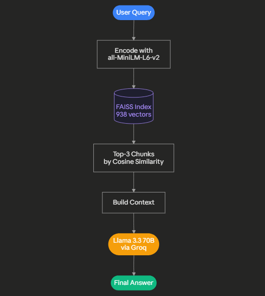
Vanilla RAG strategy for my experiment

Vanilla RAG is the baseline, and understanding how it’s working is even easier: So first it encodes the query, after that searches FAISS for the most similar chunks, then retrieves the top-3, and finally generates an answer.

def retrieve_vanilla(query: str, top_k: int = 3):
    q_emb = embedder.encode([query]).astype("float32")
    faiss.normalize_L2(q_emb)
    scores, indices = faiss_index.search(q_emb, top_k)
    return indices[0].tolist(), scores[0].tolist()

I ran my experiment with 30 queries, and the result is here:

• The average cosine similarity score was 0.6397

• Average latency was 0.10s per query

I also found out that on direct and focused queries, it was remarkably confident:

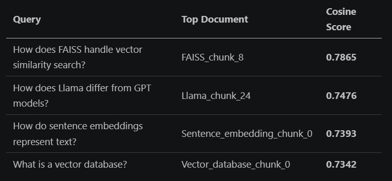
Vanilla RAG confident retrievals

It gave me clean and high-confidence retrievals. The right document surfaced immediately.

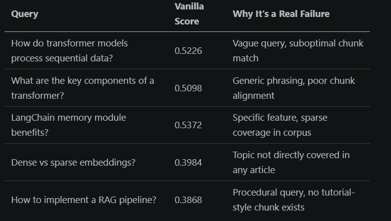
The failures were equally clear. On vague or procedural queries, the scores dropped sharply:

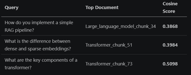
Vanilla RAG Poor Retrieval

I also saw some scores below 0.40, which means they are genuine retrieval failures. These are the queries a self-corrective system should catch and fix. For now, keep that number in mind — I will come back to it.

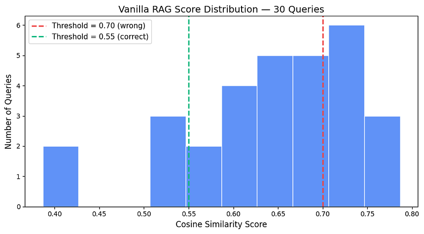
Score distribution over 30 queries

Strategy 2 — Hybrid RAG: The Quietly Useful One

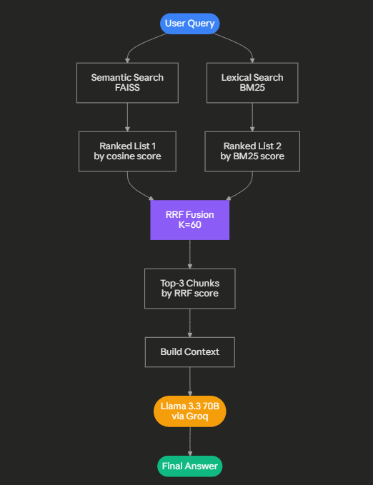
Hybrid RAG strategy for my experiment

So when we talk about Hybrid search, it runs two retrieval engines in parallel:

1. BM25 for exact keyword matching

2. FAISS for semantic similarity

After that, it fuses their rankings using Reciprocal Rank Fusion (RRF):

def retrieve_hybrid(query: str, top_k: int = 3):
    K = 60  # Standard RRF constant

    # BM25: keyword-based ranking
    bm25_scores = bm25.get_scores(query.lower().split())
    bm25_ranked = sorted(range(n), key=lambda i: bm25_scores[i], reverse=True)

    # FAISS: semantic ranking
    sem_ranked = faiss_index.search(q_emb, n)[1][0].tolist()

    # RRF fusion: reward documents that rank high in BOTH lists
    rrf = {}
    for rank, idx in enumerate(bm25_ranked):
        rrf[idx] = rrf.get(idx, 0) + 1.0 / (K + rank + 1)
    for rank, idx in enumerate(sem_ranked):
        rrf[idx] = rrf.get(idx, 0) + 1.0 / (K + rank + 1)

    return sorted(rrf, key=rrf.get, reverse=True)[:top_k]

The result: Hybrid and Vanilla disagreed on 19 out of 30 queries.

Well, I can't say that’s a small variation. It clearly indicates that BM25’s keyword signal was pulling in genuinely different documents on 63% of queries. 

In many cases, those different documents were clearly better; see some results below:

Query 1. “What makes large language models prone to hallucination?”

• Vanilla retrieved: Large_language_model_chunk_95

• Hybrid retrieved: Hallucination_chunk_16 ✅ — the directly relevant article

Query 2. “How do you implement a simple RAG pipeline?”

• Vanilla retrieved: Large_language_model_chunk_34

• Hybrid retrieved: Retrieval-augmented_generation_chunk_9 ✅ — the right source

Query 3. “How can you mitigate hallucinations in LLMs without retraining?”

• Vanilla retrieved: RAG_chunk_23

• Hybrid retrieved: Hallucination_chunk_75 ✅ — more specific

In all three cases, BM25 caught what semantic search missed. This is the gap hybrid search fills.

And the cost latency was nearly zero.

Hybrid averaged 2.03s per query in this run — most of that was the LLM call, not the retrieval. The BM25 + RRF step added milliseconds.

Strategy 3 — Self-Corrective RAG: The System That Worked Against Itself

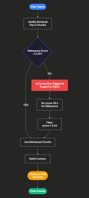
Self-Corrective RAG strategy for my experiment

Self-corrective retrieval means the system checks if the documents it retrieved are actually relevant to what the user asked.

If the relevance scores are too low, it assumes the search failed and tries a better search by expanding the query.

This helps RAG systems find better answers and reduces incorrect or hallucinated answers.

def retrieve_self_corrective(query, top_k=3, threshold=0.70):
    indices, _ = retrieve_vanilla(query, top_k)

    # Score each doc against the query
    rel_scores = [(idx, cosine_sim(query, documents[idx])) for idx in indices]
    max_relevance = max(score for _, score in rel_scores)

    if max_relevance < threshold:
        # Correction triggered — expand to top-6 and re-score
        indices, _ = retrieve_vanilla(query, top_k=6)
        rel_scores = [(idx, cosine_sim(query, documents[idx])) for idx in indices]

    filtered = [(idx, s) for idx, s in rel_scores if s >= threshold * 0.6]
    return filtered[:top_k]

During this phase of my experiment, I set the threshold at 0.70. Just to see how it will affect the result.

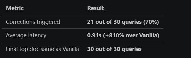
Self-Corrective RAG result at threshold 0.70

The result was shocking. Its average latency increased by +810%, still I see the same result what i saw in the vanilla rag section, zero improvement in retrieval. 

The system was triggering corrections on queries like:

•  “What is LangChain used for?” (score: 0.7195)

• “How does Hugging Face contribute to open-source AI?” (score: 0.7160)

They are those queries where vanilla RAG had returned the correct document on the first try.

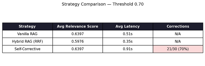
Strategy Comparison at Threshold 0.70

With this result, I can say I made a system that did not trust itself.

The Fix: One Number

Let’s have a look at the distribution from vanilla RAG across 30 queries:

Score Range and Queries Breakdown

My threshold of 0.70 was flagging the entire “decent” range as failures.

Those 18 queries with the score range 0.55 to 0.69 were retrieving the right documents. Well, not with sky-high confidence scores, because 500-character Wikipedia chunks and a lightweight embedding model have a natural ceiling.

Till now, I thought that there might be something wrong with the threshold, so I changed one line:

# Before
threshold: float = 0.70

# After
threshold: float = 0.55

What Happened When I Lowered the Threshold

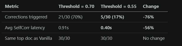
Self-Corrective RAG result at threshold 0.55

Still, I found 5 corrections that remained at the 0.55 threshold. And those were genuinely weak retrievals:

5 genuinely weak retrievals

These are the queries worth spending extra compute on. 

The other 25?

Well, Vanilla RAG had already found the right document. Previously the self-corrective layer was just burning time, confirming what was already correct. But now we have a nearly perfect result.

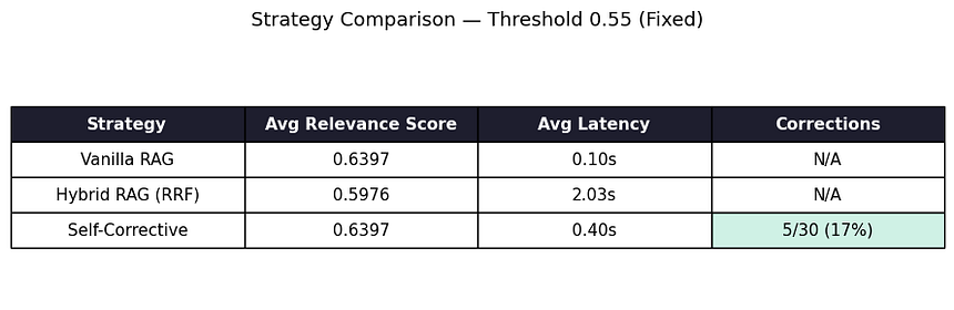
Strategy Comparison at Threshold 0.55

The Calibration Lesson

Threshold is not something that one size fits all. It is a function of three things, and you should pay attention to each of them:

1. Your embedding model.

Smaller models like all-MiniLM-L6-v2 produce lower absolute cosine scores than larger models. A score of 0.65 from this model might represent the same retrieval quality as 0.80 from a larger model.

2. Your chunk size. 

Smaller chunks produce lower scores because there is less semantic overlap with the query. My 500-character chunks were always going to score lower than 1500-character passages.

3. Your domain. 

A clean, well-structured corpus like Wikipedia will produce higher scores than a messy enterprise knowledge base of PDFs and Slack exports.

How to calibrate properly:

I follow these 4 steps. Because after this experiment, I realized this is the correct way to handle the calibration properly. If you follow these 4 steps, then this will be a piece of cake:

Step 1 — Run vanilla RAG on 30–50 representative queries from actual use case. Record every cosine score.

Step 2 — Manually label each retrieval as: good (right document), acceptable (related document), or bad (wrong document).

Step 3 — Find the score at which “bad” retrievals cluster. Set your threshold there — not at the boundary between “excellent” and “good.”

Step 4 — After deployment, monitor your correction rate. If it exceeds 20–25% of queries, your threshold is too high. Corrections should catch edge cases, not serve as a second opinion on every request.

In my case, the right threshold was 0.55, which reduced the correction rate from 70% to 17%. It catches only the genuinely weak retrievals while leaving well-performing queries untouched.

Final Comparison: All Three Strategies

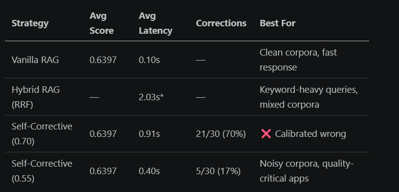
Final Result

Hybrid latency dominated by LLM call in this run; retrieval itself adds milliseconds.

My Verdict

If you are building a RAG system today, here is the order I would follow:

Start with Vanilla RAG. 

Your primary goal should be to understand what your baseline looks like before you optimize anything. First Run 30 queries, look at the score distribution, and identify where it fails.

Add Hybrid Search next. 

It is nearly free in terms of latency, requires no additional infrastructure, and the BM25 signal meaningfully improves retrieval on keyword-specific queries.

 In my experiment, it chose a different — and often better — top document on 63% of queries.

Add Self-Corrective RAG only when you have calibrated your threshold on real data. 

The mechanism works. But deploying it with an arbitrary threshold does not make your system smarter — it makes it paranoid. 

Spend 30 minutes plotting your score distribution before writing a single line of correction logic.

Reproduce This Yourself

All you need:

pip install langchain-groq faiss-cpu sentence-transformers
pip install rank-bm25 wikipedia-api pandas tabulate colorama

Free Groq API key at console.groq.com. The GitHub repo is here. 

I recommend you try running it with threshold values of 0.45, 0.55, 0.65, and 0.75. Watch how the correction rate changes. That four-run comparison will teach you more about calibration than anything written here.

References

[1] Yan et al., Corrective Retrieval Augmented Generation (2024), arXiv:2401.15884

[2] Robertson & Zaragoza, The Probabilistic Relevance Framework: BM25 and Beyond (2009), Foundations and Trends in Information Retrieval

[3] Johnson et al., Billion-scale similarity search with GPUs (2019), IEEE Transactions on Big Data — FAISS

Frequently Asked Questions

What is a self-corrective RAG system and how does it work?

A self-corrective RAG system, inspired by CRAG (Corrective Retrieval-Augmented Generation), uses a relevance gate to score retrieved documents after retrieval. If the confidence score is too low, the system automatically expands the search and tries again to find better results.

What was the main problem the author discovered in their self-corrective RAG implementation?

The author's relevance gate threshold was set incorrectly, causing the system to trigger corrections on 21 out of 30 queries (78% extra compute) while still returning the same documents as vanilla RAG every single time.

What dataset and tools were used in this self-corrective RAG experiment?

The experiment used 15 Wikipedia articles on AI/ML topics split into 938 chunks, FAISS and BM25 for indexing, the all-MiniLM-L6-v2 embedding model, and Llama 3.3 70B via Groq API for generation—all free tools.

How does vanilla RAG differ from self-corrective RAG?

Vanilla RAG simply encodes the query, retrieves the top documents from the index, and generates an answer without any relevance checking. Self-corrective RAG adds a relevance gate that evaluates retrieval quality and can trigger additional searches if confidence is too low.

What was the average relevance score for vanilla RAG in this experiment?

The vanilla RAG baseline achieved an average cosine similarity score of 0.6397 across the 30 test queries.

Why did the author choose Wikipedia articles for this experiment?

Wikipedia was chosen because it provides structured, factual content that is freely licensed for commercial use, making it ideal for testing retrieval systems.